This is my personal summary of the lecture "Web Mining" hold by the CSSH at the RWTH Aachen in the summer term of 2019. The structure of this document is based on the structure of the lecture. My goal was not to copy the slides but provide an easy to read document which contains the key information of the lecture and helps prepairing for the exam.

---

Introduction

A general definition of the web mining:

Web mining is the use of data mining techniques to automatically discover and extract information from Web documents (R. Kosala, 2000)

Web Mining splits into 3 main fields. All 3 of them are covered in some way in this lecutre.

• Web Content Minng

  • Detect regularities in unstructured content (e.g. HTML)
  • Categorize/Cluster/Classify websites
  • Application of text mining

• Web Structure Mining

  • Analyze the links between websites and effects
  • Application of network analysis

• Web Usage Mining

  • Analyze user behavior on the web

Goals of this course are to understand search engines, algorithms for finding access patterns, statistical model for user behavior and gain practical experience in web mining with python.

Statistics

We need to define some statistic measurements, which are used during this coures.

Mode: Most frequent value
Mean: Expected value $E[X]$, also written as $\bar{x}$ or $\mu$
Median: Value that separates lower and higher half of values
Variance: Measure of spread: $V = \frac{1}{n} \sum_{i=1}^{n} (x_i - \bar{x})^2$
Standard deviation: $\sqrt{V}$
Maximum likelihood: Choose the parameter which maximize the likelihood

A statistical model embodies assumption how the data is generated in a probabilistic way.

Overview of statistics for programmers

Optimization

Gradient descent (GD): Minimize a function: $f(x) = f(x) - f'(x)$. Start at a random x and step towards the x with $f'(x) = 0$.
Convex-Function: For this speacial functions the gradient descent will find the global minimum scrapper Stochastic gradient descent (SGD): Faster to compute then the complete gradient, but will not converge as for $f'(x)$ there will be a $a$ so that $y=y-a*f'(x)$. $a$ is called the learing rate a

How does the internet work

Internet vs WWW: Internet $\neq$ WWW. The internet describes a network of many computer networks, which exchange data. The WWW, in the meaning of websites/documents with URLs and hyperlinks, is one possible use case for this. Others are for example streaming and emails.

OSI model: Open Systems Interconnection Model - Organizes services between clients in a network

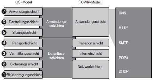
Transport oriented layers: Network layer (IP network protocol); Transport layer (TCP-IP protocol); Physical layer (Transmission of raw bits); Data link layer (Mac address, PPP connection)
Application oriented layers: Session layer; Presentation layer (Encryption, Compression); Application layer (Interface to end-user)

We have basically 2 options to receive a lot of data from a website:

• Web scraping

  • Request HTML pages
  • Extract information
  • Disadvantages: Parsing is difficult, lass efficent and can break down by little changes; Web scraper can be blocked
  • Advantages: Get all information a user can see, less restricted, API are not always avaible

• Web services/API's

  • Client-Server architecture
  • Return format XML/JSON

OAuth: Open auth protocol

Web Search & Information Retrieval

Spidering: Bots/Crawlers recursively follow linked websites from given Start-URLs
Sitemaps: XML which informs crawlers about avaible URLs from the website
robots.txt: Inform web crawlers which files/folders are allowed for crawling. The crawler is not bound to this
Bot detection: CAPTCHA, honeypot Preferential crawlers: Give unvisited link a priority

Inverted Index

Document 1: Hans is a goat.
Document 2: A goat is an animal ... goat.

Simple inverted index: Hans: $id_1$; ... ; goat: $id_1, id_2$; is: $id_1, id_2$; anmial: $id_2$; ...
More complex inverted index: Hans: $<id_1,1,[1]>$; ... ; goat: $<id_1,1,[4]>, <id_2,2,[2,x]>$; is: $<id_1,1,[2]>, <id_2,1,[3]>$; ...

The inverted Index can be stored in a large hashtable

Web Content Mining

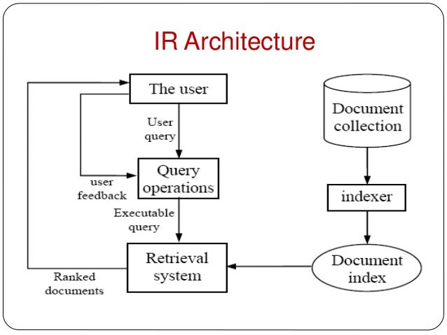
Information Retrieval

Finding relevant documents (web pages) to a given user query, for example with web search. In difference to normal data retrieval we don't have a ordered/structured database and no query language like SQL to retriev data. The found documents are than going to be ranked according to their relevance for the user.

Web search is different to traditional IR:

• Efficiency is more important
• Web pages differ from pure text
• Spamming is a issue on the Web

Information retrieval models

Describes how a document/query is represented and the relevance of a document for a given query

Boolean Model

• Simplest IR model based on boolean algebra (AND, OR, NOT)
• The documents for which the query is locial true will be retrieved

A = Brutus; B = Caesar; C = Calpurnia

	Hamlet	Othello	Macbeth
A	1	0	0
B	1	1	1
C	0	0	0

Brutus AND Caesar AND NOT Calpurnia
100 AND 111 AND NOT 000 $\rightarrow$ 100

Vector Space Model

• Most widely used IR model

Document-Term Matrix: $n \times m$ matrix with the frequency of the n Terms in each of the m documents
Term Frequency (TF): $tf_{ij}= \frac{f_{ij}}{max\{f_{1j},...,f_{|V|j}\}}$
$f_{ij}$ is the number how often Term i appears in Document j
Inverse document frequency (IDF): $idf_i = \log \frac{N}{df_i}$
$N$: number of documents; $df_i$: number of documents where $t_i$ appears
TF-IDF: $w_{ij} = tf_{ij} * idf_i$
Term weight: $w_{iq} = (0.5 + \frac{0.5f_{iq}}{max\{f_{1q},...,f_{|V|q}\}})*idf_i$ of term $t_i$ in query q

Advantages:

• Partial matching (even when no document contains every term)
• Ranking similarity
• Term weighting

Statistical Language Model

Every term is considered individually (unigram). Documents are ranked by the likelihood of the query given the document.

$Pr(q=q_1 q_2 ... q_m | d_j) = \overset{|V|}{\underset{i=1}{\prod}}Pr(t_i | d_j)^{f_{iq}} = \overset{|V|}{\underset{i=1}{\prod}} (\frac{f_{ij}}{|d_j|})^{f_{iq}}$

Evaluation Measures

Are retrieved documents relevant and are all relevant documents retrieved?

Precision at position i: $p(i)=\frac{\text{Number of relevant documents until i}}{i}$
Recall: $\frac{\text{Number of relevant documents until i}}{\text{Number of all relevant documents}}$
Average Precision: $p_{avg}=\frac{\sum p(i)}{\text{Number of all relevant documents}}$

Text and web page preprocessing

This includes stemming, stopword removal, HTML tag removal,... to make a documents shorter and queryable.

Indexing documents for retrieval

Latent Semantic Indexing

Also called LSI has the goal to identify association of terms. This is achieved by reducing the dimensions of an n-dimensional term space. With this it is possible to see different meaning of terms in the context of other terms.

Eigenvalue($\Lambda$) and Eigenvector($v$): $\text{S}v = \Lambda v$

Singular Value Decomposition

Factor a matrix A ($m \times n$) into 3: $A = U \Sigma V^T$ with

Here is a good example on SVD.

This reduces the dimensionality of the rank and this is the mathematically optimal of reducing dimension.

k-concept space: Consider the k largest singular values and set the remaining values to zero
$A_k = U_k \Sigma_k V_k^T = U \text{diag}(\sigma_1,...,\sigma_k,0,...,0) V^T$

The k-concept space is an approximation with an error of $\sigma_{k+1}$ as this is the next value which is excluded from the k-concept space.

All in all the LSI performs better than tradional keywords based methods and has proved to be a valuable tool for natural language processing as well as in information retrieval. The time complexity of SVD is high ($O(n^{2k^3})$). This can reduced by a k-concept space, but there is no fixed optimal k. It has to be found first (normally around 150-350 words). Also SVD assumes data to be normally distributed.

Metasearch

Combining search enginge to increase coverage while not having an own database.

Combination using similarity score:

• CombMIN($d_i$) = $min\{ c_1(d_1),...,c_n(d_1)\}$
• CombMAX($d_i$) = $max\{ c_1(d_1),...,c_n(d_1)\}$
• CombSUM($d_i$) = $c_1(d_1)+...+c_n(d_1)$
• CombANZ($d_i$) = $\frac{c_1(d_1)+...+c_n(d_1)}{n}$

Combination using ranking positions:

• Borda ranking: For every search engine each of the n documents get a number starting with the highest rank getting the number n and the second highest getting n-1 and so on. When there are unranked pages for the search engine the remaining points are divided.
• Condorcet ranking: ...
• Reciprocal ranking: Same principal as Borad ranking but with fractions - The highest ranked document gets a $1$ and the second one gets a $\frac{1}{2}$ and so on. Calculate the sum of the reciprocal rankings for each item and compare them: $Score(a)=1+...+\frac{1}{2}=2,3$

The ranking is written as a set in descending order.

Web Structure Mining

Strongly connected: For a graph there is a path between every pair vertices $\rightarrow$ strongly connected component is a subset, which is strongly connected

PageRank

Simulate behaviour of a random surfer to rank every web page by likelood that it will be visited.

Transition matrix: stochastic matrix M
Calculating a step: One step: $M * v_0$; k-steps: $M^k*v_0$
The goal is to have an equation $v=Mv$. The eigen vector $v$ tells us on which page the surfer most likely ends up.

Bow tie structure of the Web

PageRank would have worked if the web was strongly connected.

Dead ends: A page which does not link to another page. If you would use the transition matrix it would not be stochastic any longer. You could delete all dead ends and incoming arcs.
Spider traps and taxation: A set of node with no arc outside and no dead end. Solution: Allow to let a surfer teleport to a random page/ start a random sufer from a new page with a small pobability: $v' = \beta M v + (1- \beta) \frac{e}{n}$

Topic sensitive PageRank creates a vector of the topics biasing the PageRank into selecting pages from specific topics. This can be usefull when you know the topics the user is interessted in.

Biased Random Walk: The topic is identified by the topic sensitive PageRank thats why now we can redirect a random surfer to a document of the topic T. $v' = \beta M v + (1- \beta) \frac{e_S}{|S|}$ with S as a set of documents identified to be related to to topic T and $e_S$ a vector, which is 1 for the components in S and otherwise 0.

Link spam

Spam farm: A collection of pages, which want to increase the PageRank of a single target page.

Search engines need to detect link spam. This is possible by looking for structures like spam farms and then eliminate the target and releated pages. This is not enough as sapmmers come up with different structures. Another solution are modifications of the PageRank.

• TrustRank: Topic sensitive PageRank with a set of trustworthy pages for those topics. Those won't link to spam pages. Humans can select trustworthy pages or pages with controlles top-level domains (.edu, .gov ...) might be a good choice as well.
• Spam Mass: $\frac{\text{PageRank} - \text{TrustRank}}{\text{PageRank}}$ ($\leq 0$ values are unlikely to be spam)

HITS

Hyperlink-Induced Topic Search

Link matrix: $L = \begin{pmatrix} 0 & 1 \\ 0 & 0 \end{pmatrix}$ if there is only a link from e.g. page a to b. $L^T$ is in the same order as the PageRank Matrix M.

Hubs: Links to pages where you can find information about a topic

• Hubbiness: $h = \lambda L a = \lambda \mu L L^T h$ - How good are the linke authority pages?

Authorities: Pages, which provide information about a topic

• Authority: $a=\mu L^T h = \lambda \mu L^T L a$ - How good are the hubs that pointed at this authority?

HITS can be used for identifying communities. This can provide information about the users interest to better target ads as well as giving insights about the evolution of the web.

Strongly connected bipartite subgraphs

Websites which are releated don't link at each other (e.g. Apple to Microsoft), but Websites who link to a page might link to several pages of this topic.

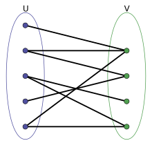
Bipartite core: Every page from a subset in U links to every page in a subset in V.

For web communities we are mostly interessted in finding the core. These can be done by pruning unqualified pages with a high in-degree of links (e.g. Google, Yahoo) or a low out-degree below a set value. For generating the core we use the apriori algorithm.

Maximum flow communities

Find the maximum flow between source s and sink t. The maximum flow can be find using the Ford-Fulkerson algorithm. Within the detected communities those with the most links to pages in the community are ranked highest. Those are then added to the source set. Repeat the algorithm to get larger communities. Maximum flow = minimum cut

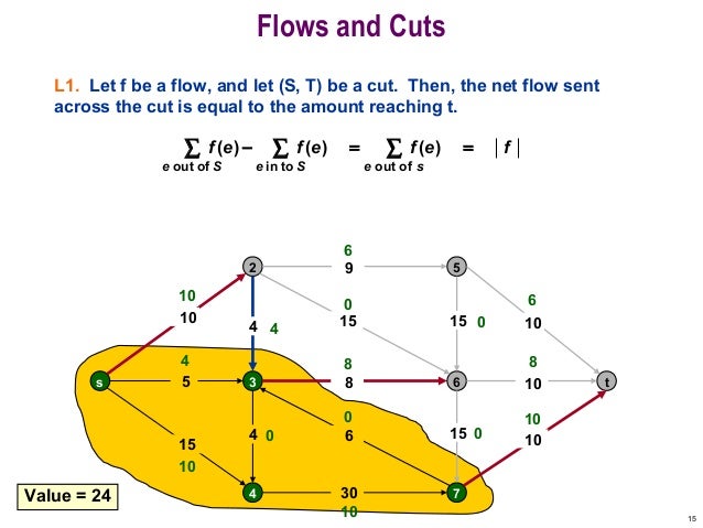
When considering the web cutting the edges would lead to two seperated web communities.

Association Rule Mining

Find associations and correlations of items and discover non-trivial and interesting associations in a data set. The most important association rules are knonw, but the detecting the unknown rules can be interessting.

Association Rules - AR

TID	Items
T1	bread, jelly, peanut-butter
T2	bread, peanut-butter
T3	beer, bread

For itemsets:
Support Count: $\sigma(\{ \text{bread}, \text{peanut-butter} \}) = 2$
Support: $s(\{ \text{bread}, \text{peanut-butter} \}) = \frac{2}{3}$
Frequent Itemset: Itemset with higher Support than a minimum support

For rules: Rule: $X \Rightarrow Y$
Support: $s=\frac{\sigma(X \cap Y)}{\text{number of transaction}}$ - frequency of the rule
Confidence: $c= \frac{\sigma(X \cap Y)}{\sigma(X)}$ - Support count of both itemsets together compared to support of X

Apriori

Most influential association rules miner. It will find the frequent itemsets (1) and from this generate rules (2).

Aprori principle: If an itemset is frequent $\rightarrow$ subset of the itemset is frequent.
$(X \subseteq Y) \Rightarrow s(X) \geq s(Y)$

With the aprori principle we can discard itemsets as soon as a subset is below the threshhold of the minimum support.

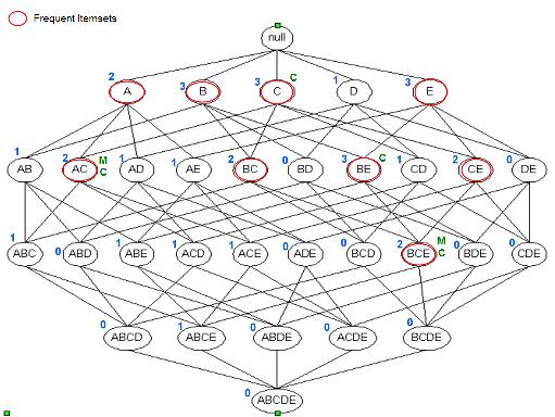
(1) From this we can simulate a aprori run and find the most frequent itemsets with $\text{minsup}= 2$:

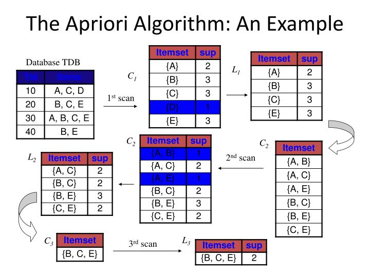
(2) The frequent itemsets help to generate association rules. For an frequent itemset L and a subset $F \subset L$ all rules $F \Rightarrow { L-F } which fullfill the minimum confidence are possible rules.

The algorithm will then output a list of association rules.

A strong association rule is a rule, which has a higher support and confidence than a given minimum threshold. Apriori algorithm produces a lot of rules from which many are redundant/uninteresting/uninterpretable. Strong rules are not equivalent to interessting rules. A strong association rule is a rule, which has a higher support and confidence than a given minimum threshold. Apriori algorithm produces a lot of rules from which many are redundant/uninteresting/uninterpretable. strong rules are not equivalent to interessting rules. A rule $A \Rightarrow B$ is interessting if $s(A,B)- (s(A) * s(B)) > 0$.

Subgroup Discovery

Identify descriptions for subsets in a dataset, which have a interesting deviation from the pre-defined concept of interest.
In difference to association rule mining subgroup discovery measures the interestingness and does not focus on confidence and support.

Subgroup discovery task: $S=(D,\Sigma,T,I,k)$
D: Dataset; $\Sigma$: Search space; T: Target concept; Q: Selection criteria; k: result set size

Interestingness measures: $q(P) = i_P^a *(\tau_P - \tau_0)$
i: Number of Instances; $\tau_P$: Target share in subgroup; $\tau_0$: Target share in entire dataset

For numerical target value $\tau$ can be replaced with $\mu$ which are the targe value of the subgroup and the entire dataset.

A strong association rule is a rule, which has a higher support and confidence than a given minimum threshold. Apriori algorithm produces a lot of rules from which many are redundant/uninteresting/uninterpretable. strong rules are not equivalent to interessting rules.

Efficient Subgroup Discovery

Pruning: If specializations of a subgroup will not achieve a high enough score to be included, they don't have to be explored

Optimistic Estimates: $oe(P) = i_P * (1-\tau_0)$ with $tau_P = 1$
Evaluate each subgroup. The best are added to a set M. If $oe < min. quality in M$ all specializations can be skipped.

Recommender Systems

Broadly used for news, videos, online-shopping, etc. The benefits for the customer are a pre-selection of things they might like as well as discovering new things. The platform can increase the customer loyalty and sales. The recommender system can be understood like a function which gives you for a user, an item and background knowledge the relevance score of this item.

Evaluation:
The recommender system does a good job, if it recommends widely unknown items that the user might like.
$\text{Precision} = \frac{ | \text{good movies recommended} | }{ | \text{all recommendations} | }$
$\text{Recall} = \frac{ | \text{good movies recommended} | }{ | \text{all good movies} | }$

Recommenders

• Basic Recommendations: Hand curated - Simple (Most views/purchases) - Not tailored to individual users

• Content-based recommonder: Recommend user x similar items to those they liked

  • Item profile: Each item has a profile with important information
  • User profile: Weighted average of rate items
    $\rightarrow$ Prediction: $u(c,i)=cos(c,i)=\frac{c*i}{ || c || * || i || }$ for user c and item i
  • Advantages: Can recommende new items - Does not require user data
  • Disadvantages: No recommandations for new users - Finding righ features is difficult

Similarity

Jaccard Similarity: $J(A,B)= \frac{|A \cap B|}{|A \cup B|}$ (No rating)
Cosine similarity: $\cos(d_j, q)= \frac{<d_j, q>}{||d_j|| \times ||q||} = \frac{ \underset{ n \in N }{ \sum } d_{ji} * q_i }{ \sqrt{ \underset{ n \in N }{ \sum } d_{ji}^2 } \sqrt{ \underset{ n \in N }{ \sum } q_i^2 } }$ (missing ratings are negative)
Pearson correlation coefficient:
$sim(x,y) = \frac{ \underset{ i \in I_x \cap I_y }{ \sum } (r_{ xi } - \bar{ r_x } )( r_{ yi } - \bar{ r_y } ) }{ \sqrt{ \underset{ i \in I_x \cap I_y }{ \sum } ( r_{ xi } - \bar{ r_x } )^2 } \sqrt{ \underset{ i \in I_x \cap I_y }{ \sum }( r_{ yi } - \bar{ r_y })^2 } }$
(Consider only ratings if user x and y rated the item; $\bar{r_x}$ is the average rating of items by user x)

Collaborative Filtering

User-based:

Prediction based on pearson correlation and the average ratings of each user:
$pred(x,i) = avg(r_x) + \frac{ \underset{n \in N}{\sum} sim(x,n) *(rn_i - avg(r_n))}{\underset{n \in N}{\sum} sim(x,n)}$

The prediction can be used to rank the items for the user (might lead to too many niche items, which can be prevented by considering the popularity)d

Items-based:

Rate the similarity between items. This can be done with cosine similarity. This often works better, as items are simpler than user. On the other hand there is the problem of what to recommend to a new user as they did not ranked anything or just a few items and what is about new, not yet rated items?

Advantages: Works for all types of content - no background info needed Disadvantages: Not rated item can't be recommended - Needs several ratings by the same user - Recommandations are not really unique for a user

Latent Factor model:

Matrix of hidden factors for each item Q and matrix of how important each factor is for each user $P^T$ leads to the complete rating matrix R: $R= Q*P^T$

Rating of a item i of user x: $r_{xi} = q_i * p_x$ ($q_i$: row i in Q; $p_x$: column x of $P^T$)

Sequential Data

Preprocessing: The data from a data source (e.g. Cookies, Web Server Logs, Web APIs,...) needs to be preprocessed to work with it. Therefor remove unusable data and find interesting identifier (e.g. IP of user).

• Sequence Clustering

  • Based on sequence similarity - extract features first

• Sequence Classification

• Sequence Prediction
• Sequence Labeling
• Sequence Segmentation

Markov chains

Sequences are transitions between states.
First order Markov chains: Memoryless - next state only depends on current one

State space: $S=\{s_1,s_2,...,s_m\}$
Markov property: $P(X_{t+1} = s_j | X_t = s_{i_t}) = p_{i,j}$
Transition martix = $M = \begin{bmatrix} p_{1,1} & ... & p_{1,j} \\ ... & ._. & ... \\ p_{i,1} & ... & p_{i,j} \end{bmatrix}$ with single transition probabilitys $p_{i,j}$ and $\underset{j}{\sum}p_{i,j} = 1$ and $p_{i,j} = \frac{n_{i,j}}{\underset{j}{\sum} n_{i,j}}$
Likelihood: $P(D|\Theta) = p(x_1) \underset{i}{\prod}\underset{j}{\prod}p_{i,j}^{n_{i,j}}$ with $n_{i,j}$ the number of transitions from i to j
Maximum Likelihood: $L(P(D|\Theta))= log(P(D|\Theta)) = log(p(x_1)) + \underset{i}{\sum}\underset{j}{\sum}n_{i,j} log(p_{i,j})$
Prediction: $(0 1) M^k = (a b)$ a and b are the predicted propabilities after k iterations, if we started from the 2nd state. This is an example if there are 2 different states.

Reset states mark the start and end of a sequence and are necessary when having multiple sequences. This means that there has to be a row and column for reset states if there are multiple sequences.

k-th order Markov chain: $x_i$ dependds on k previous states

Bayesian Statistics: $P(A|B)=\frac{P(B|A)P(A)}{P(B)}$

Sequential Pattern Mining

"Given a set of data sequences, the problem is to discover sub-sequences that are frequent, i.e., the percentage of data sequences containing them exceeds a user-specified minimum support" [Garofalakis, 1999]

PrefixSpan

Complete example which explains it clearly.

Advantages: No explicit candidatae generation (in oposite to apriori) - Projected databases keep shrinking
Disadvantages: Construction of projected database can be cost intensive

Sparse data tends to favor the PrefixSpan Algorithm.

Misbehaviour on the Web

Types of Misbehavior:

• Malicious users: Trolling, Vandals
• Misinformation: Hoaxes, Fake reviews

Goal is to analyze this misbehaviour.

Trolling

Trolls disrupt online discussion. They make regular users feel uneasy or make them leave a discussion. The troll is correlated to a psychopathic, narcissistic and sadistic personality. From the behavior he acts less positive, less on topic, post more per thread, uses more profane language and with all this receives more replies/attention. A negative mood and a negative context effects trolling by increasing the trolling behavior. Trolls who receive negative feedback are likely to troll more.

What to do against trolls

• Discourage negative feedback (no dislike button)
• Delete troll/ negative comments
• Disallow too quick posts
• Shadow banning: Comments of trolls are not visible to anyone else
• Hellbanning: Comments of trolls are only shown to other trolls

Sockpuppet

A fake account run either part of a network of sock puppet accounts or just by itself run by one person (UrbanDictionary)

Used for diversify, anonymize, multiply identity or privacy.

Detect sockpuppets:

• Similar usage than other users
• Login time, login IP address, username, point of view, supports particular user
• Used more often in controversial topics
• Start fewer discussions
• More opinionated, upvote each other more, are downvoted more

Vandals

Vandalism is“an action involving deliberate destruction ofor damage to public or private property.”

More likely to quickly edit (e.g wikipedia) pages and having a decreasing amount of edits over time. They can be detected by there meta data (registered, account-age, edit quantity, block history, ...) or content driven by trusting all content that survived multiple edits more.

Misinformation

We differ between misinformation by intent (Disinformation) and by knowledge (Fake reviews, hoaxes).

Detect misinformation

• Manual inspection
• User ratings/ Feedback
• Duplicates
• Unexpected rule (Always negative, except for one really positive review)
• Cluster users into categories

Open Problems in detection: Early detection of misbehavior, coordinated attacks, anonymity vs single verified identity

Representation learning

...

Handling Large Datasets

Distributed data analysis

Cluster Computing is used for huge clusters like the google cloud. Problems are the network bottleneck (due to bandwith) and complex distributed computing.

Map-Reduce

Store data redundantly (persistence and availability) and move computation close to data. Distributed File System: Chunk servers (Split files into contiguous chunks with replicates), Master node (knows where which file is stored), Client library for file access

Document will be split into key-value pairs which are than grouped by key and will be reduced, if they have appear several times.

Shingles

k-shingle: k characters that appear in the document

Common shingles $\rightarrow$ simmilar text.

Hash function

The probability that the minhash function for a random permutation ofrows produces the same value for two sets equals the Jaccard similarityof those sets

In Detail

Local sensitive hashing

Read this

Data streams

Ads

Bipartite matching

Perfect matching: Every node appears in the matching

Adwords problem

We need a online algorithm (e.g. Greedy algorithm with competitive ratio $\frac{1}{2}$)

Balance Algorithm:

A/B Test

Test Calls to action (CTA, 'buy now' vs. 'add to card') and Content (like Image vs. no Image)

Measure test: Use a statistical hypothesis test and decide on the result depending on the p-value. From the p-value you can decide weather to discard the null-hypothesis or not.

t-test: Formular here
Kolgomorov-smirnov test: Formular here

Only usefull for large data sets.

Explore vs exploit

Greedy algorithm
$\epsilon$-Greedy algorithm: is sensitive to bad tuning. Performs as good as the UCB algorithm
UCB algorithm

---

Overview

Important Formulars